How to use Cube object ?

Data cube structure

The spectro-imaging data generated by the JWST instruments respects the same characteristics as the vast majority of observations made with telescopes on Earth (e.g. ALMA, ESO/SINFONI-MUSE, etc.). Data are stored in a 3-dimensional array. Two dimensions correspond to spatial coordinates (x,y), the third dimension is a spectral dimension, by default given in microns (λ). By fixing a wavelength on the spectral axis, we extract a 2D array corresponding to an image, conventionally called a channel map.

Create a data cube using JWSToolKit

Getting started

After installing the package, simply call the module ‘Cube’ in the python code and specify the name of the file to be opened:

from JWSToolKit import Cube

file = "DataCube_s3d.fits"
cube = Cube(file)

cube.info()

cube.info() prints the information associated with the data stored in the file’s headers in the terminal. Here’s an example of the output:

__________ DATA CUBE INFORMATION __________
Data file name:DataCube_s3d.fits
Program PI: Dougados, Catherine, for the project: A cornerstone study of the jet/outflow connexion: the remarkable DG Tau B system
Program ID: 01644
Target: DG TAU B
Telescope: JWST \ Instrument: NIRSPEC
Configuration: G140H + F100LP
Number of integrations, groups and frames: 2, 20, 1
Dither strategy: True
Dither patern type: 4-POINT-DITHER

Date and time of observations: 2022-09-05 | 14:04:52.091999
Target position in the sky: RA(J2000) = 66.76086125 , Dec(J2000) = 26.09164722222222
Effecive Exposure Time: 9336.896 s
Total Exposure Time (with overheads): 9803.728 s

Data type and shape: Data Cube | 77, 67, 3915 (x, y, wvs)
Spatial pixel sizes in deg (dx, dy): 2.77777781916989e-05, 2.77777781916989e-05
Spatial pixel sizes in arcsec (dx, dy): 0.1, 0.1
Spectral pixel size (µm): 0.000235
Spectral range of observations (µm): 0.9700000000000001 - 1.89
Units of spectral pixel values: MJy/sr

In this example, and in the following description, the data presented are those from the 1644 program of Cycle 1 JWST. These data are presented and analyzed in Delabrosse et al. 2024. The first section presents general data information: the project’s ‘principal investigator’, the name of the target, the instrument used and the instrument configuration. The second section places the observations in time and space, giving the date the data was taken and the exact position of the target. The last section provides more detailed information on data parameters. For this example, the data cube has 77 and 67 pixels in the X and Y directions and has 3915 channels maps (the sampling of the spectral axis). The method provides information on pixel size, spectral sampling and the unit of cube values.

Attributes of the ‘Cube’ object

Attribut	What is it?
Cube.file_name	The name of the file in .FITS format.
Cube.primary_header	The primary header of .FITS data.
Cube.data_header	The header associated with data science (i.e. the data cube).
Cube.data	The data cube, values stored in a 3D array.
Cube.errs	Errors associated with science data, stored in a 3D array.
Cube.size	Data cube dimensions (nλ, nx, ny).
Cube.px_area	Area of spatial pixels, in arcsec^2.
Cube.units	The unit of data cube values, by default these values are surface brightnesses given in MJy/sr.

Methods of the ‘Cube’ object

Method	What does it do?
Cube.info()	Prints data-related information stored in headers.
Cube.get_wvs()	Returns the wavelength axis.
Cube.get_px_coords()	Converts R.A. Dec. coordinates in degrees to pixel coordinates.
Cube.get_world_coords()	Converts pixel coordinates to R.A. Dec. coordinates in degrees.
Cube.extract_spec_circ_aperture()	Extracts a spectrum integrated into a circular aperture.
Cube.line_emission_map()	Creates an integrated emission map under a spectral line.
Cube.rotate()	Apply a rotation using WCS.
Cube.pv_diagram()	Creates a PV diagram extracted in a horizontal rectangular slit.

Extract a spectrum in the cube

The main purpose of working with spectral cubes is to obtain spectral information at a given position in the field of view. The following example shows how to extract a spectrum inside a circular aperture:

import matplotlib.pyplot as plt

wvs_values_um = cube.get_wvs()                # Returns the wavelength axis in microns.
wvs_values_nm = cube.get_wvs(units = 'nm')  3 # Same as above, but in nanometres.

spectrum_values = cube.extract_spec_circ_aperture(radius=4, position=[25,25])  # Values in Jy

# Plot
fig, ax = plt.subplots()
ax.step(wvs_values_um, spectrum_values, color='black')
ax.set_xlabel('Wavelength (µm)')
ax.set_ylabel('Flux density (Jy)')
fig.tight_layout()
plt.show()

The Cube.get_wvs() method is used to construct the wavelength axis. By default, values are given in microns, but it is possible to choose the wavelength unit (other possibilities: Ångström or nanometers). The spectrum is constructed using the Cube.extract_spec_circ_aperture() method. A radius and a position [x,y] of the circle center in the field of view must be specified. Values are given in pixels. By default, the spectrum returned is in Jy, but you can also choose the unit of the values returned (‘Jy’, ‘erg s-1 cm-2 um-1’ or ‘erg s-1 cm-2 Hz-1’).

Convert (R.A., Dec.) coordinates

The data header stores information about the coordinate system (the World Coordinate System: WCS). It is then possible to convert coordinates (R.A., Dec.) into pixel values ​​in the cube images. Conversely, from a pixel position in the cube, it is possible to find its equivalent in the (R.A. Dec.) system.

DGTAUB_POSITION_DEG = [66.76071774, 26.09171944]    # (RA, Dec) (deg)

coords_pixels = cube.get_px_coords(DGTAUB_POSITION_DEG)
print(coords_pixels)

(array(30.5219849), array(28.9215127))

The .get_px_coords() method converts a position in R.A. Dec. (in degrees) to pixels [x,y]. It is also possible to give several positions, in which case you must give a list containing two lists: [[x1, x2, …, xN], [y1, y2, …, yN]]. Conversely, it is also possible to convert one or more positions into pixels in the R.A. Dec. coordinate system:

coords_radec = cube.get_world_coords([30,28])
print(coords_radec)

(array(66.76119783), array(26.09180495))

Apply rotation

It is sometimes useful to rotate the data cube. This can be done using the method:

cube_rotated = cube.rotate(angle=295, control_plot=True)

The rotation angle must be specified in degrees. The angle follows the same convention as the ‘Position Angle’ (PA), i.e., the rotation is counterclockwise and with the 0 degree angle aligned with the vertical North axis. The Cube.rotate() method returns a cube object, constructed like the original cube but with the modified WCS rotation matrix.

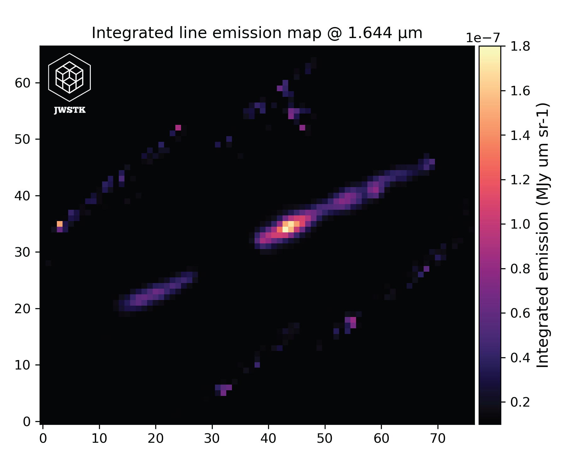
Extract an integrated emission line image

An integrated emission line map, also known as a moment 0 map, is derived from a three-dimensional data cube by summing the flux across the spectral axis over the wavelength interval corresponding to a specific emission line. This process yields a two-dimensional representation of the total line intensity at each spatial position. In the context of the JWST instruments, such maps are invaluable as they allow people to spatially resolve regions of enhanced emission, providing critical insights into the physical conditions and distribution of ionized gas in astronomical sources.

import matplotlib.colors as colors

WV_LINE = 1.64355271  #  Line wavelength (µm)
line_map = cube.line_emission_map(wv_line=WV_LINE)

fig, ax = plt.subplots()
ax.imshow(line_map, origin='lower', cmap='magma', norm=colors.LogNorm())
ax.set_xlabel('X (pixels)')
ax.set_ylabel('Y (pixels)')
fig.tight_layout()
plt.show()

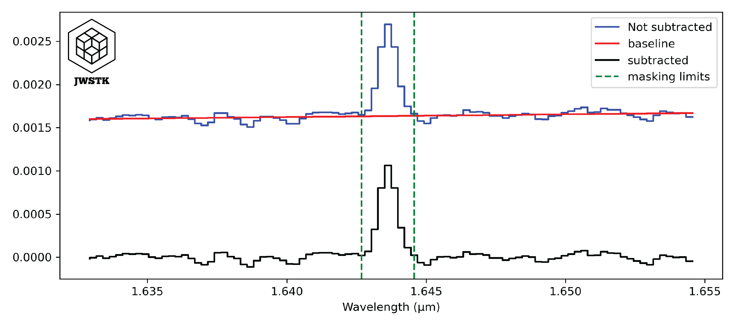
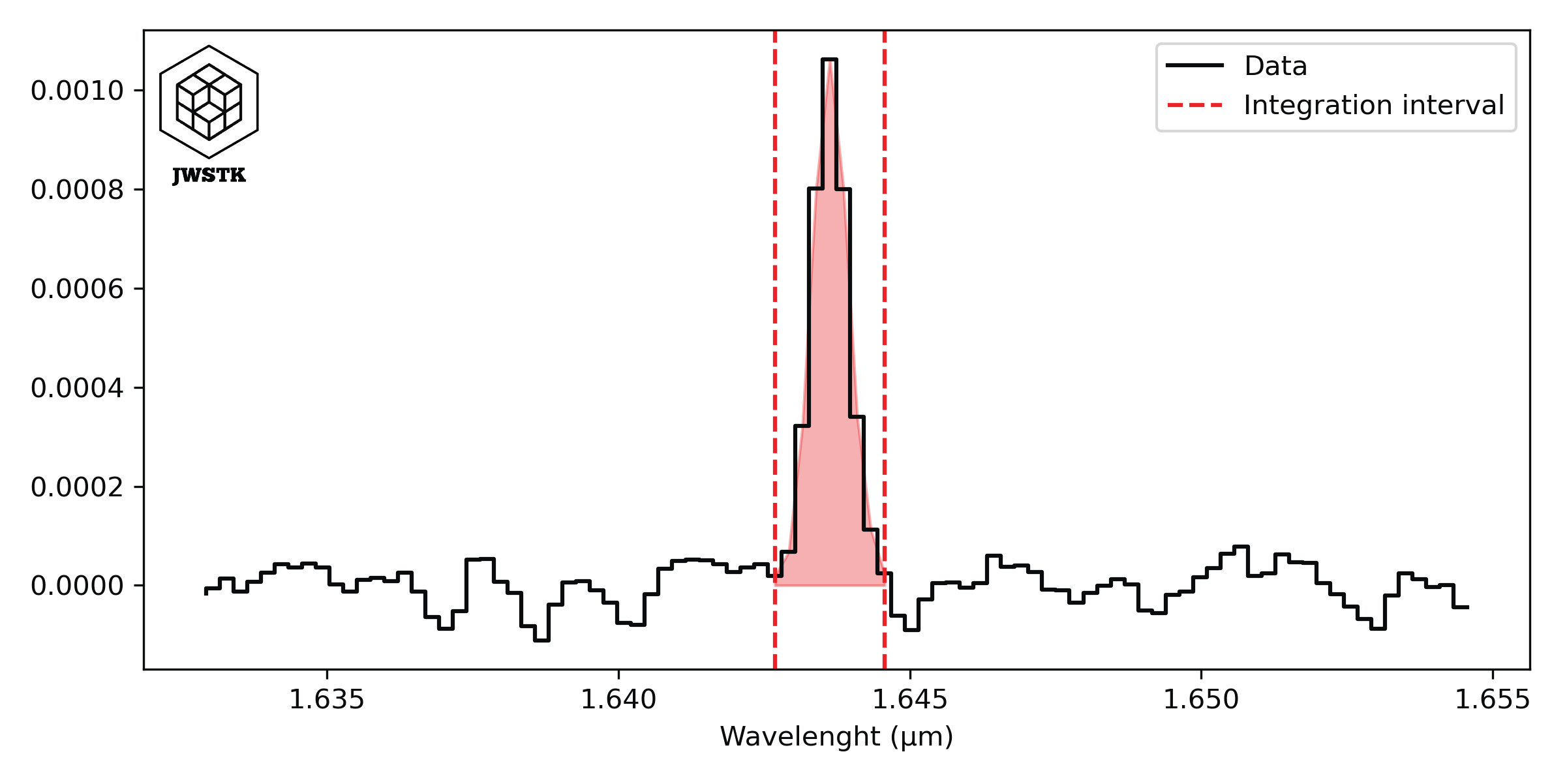
It is possible to change some parameters involved in the extraction of the emission line in the spectra. The integration of the intensity of the line is done after the subtraction of the baseline, adjusted around the line. The size of the interval can be changed with the parameter continuum_range, it will then be necessary to give the value in km/s.

Similarly, a parameter line_width corresponds to the spectral width of the emission line. By default it is fixed at 400 km/s.

The function returns a 2D array, containing the integrated values ​at each pixel. By default the values ​​are in MJy um / sr, but it is possible to choose other units (‘erg s-1 cm-2 sr-1’).

This method uses the methods included in the Spec class: Spec.cut(), Spec.sub_baseline(), and Spec.line_integ(). An example of how baselines are subtracted from spectra and how integration under the line is done are shown below:

Create a Position-Velocity diagram

A position-velocity (PV) diagram is a graphical representation that allows one to visualize the distribution of a source’s emission velocity as a function of its position in the sky. By extracting a slice along a spatial axis from a spectro-imaging cube (where the spectral axis often corresponds to velocities through the Doppler effect), this diagram highlights the internal dynamics of the observed object, revealing features such as disk rotation, matter flows, or other complex movements. Thus, the PV diagram is a valuable tool for analyzing kinematics and gaining deeper insight into the physical processes at work in astrophysical environments.

The Cube.pv_diagram() method constructs the PV diagram from several parameters. First, the emission line wavelgnth: wv_line. This value must be given in µm, for a wavelength at rest and in a vacuum. Next, you must specify the characteristics of the slit: its position in the field of view in pixels slit_position [xc,yc], its width and height in pixels slit_params [w,h].

pv_diagram = cube.pv_diagram(wv_line = WV_LINE, slit_position=[25,25],
                            slit_params=[20,4], control_plot=True)

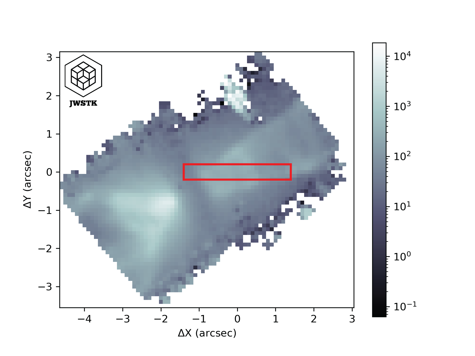
The horizontal axis of the diagram corresponds to the spatial dimension (the X axis of a slit). The vertical axis shows the wavelengths converted to radial velocity, taking the rest wavelength of the emission line as the reference for the Doppler shift. The values in each pixel of the diagram correspond to the intensities for a given X position and wavelength in the data cube. The values have the same units as those in the cube.